
Beginner · visual course

Sensors

A sensor does not simply produce truth: it converts a physical quantity into a signal that must be sampled, calibrated and checked.

I2CAnalogData logging 4 guided sessions 8 skill tracks 3 example projects
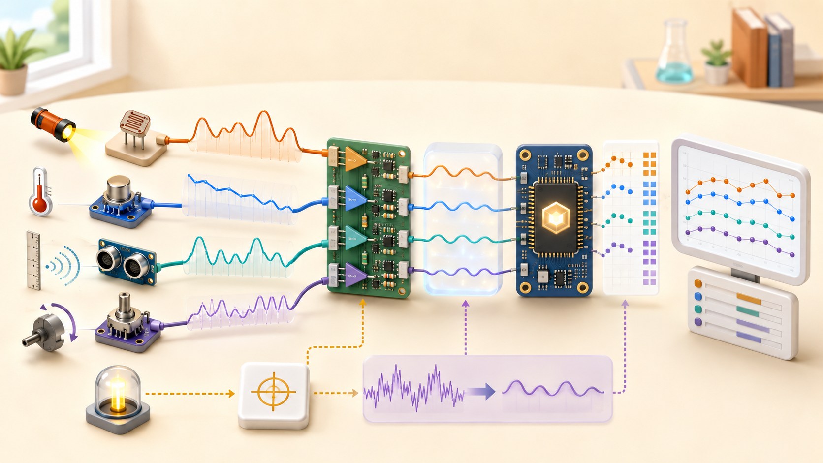
Three-dimensional educational sensor chain converting light, temperature, distance and position into calibrated digital data
Concept overview · generated for this Academy4Tech lesson
Start here

See the system, then build it.

Always record the unit, conditions and uncertainty. A number without context is not yet a trustworthy measurement.

01Trace a physical quantity through a transducer to a digital reading
02Distinguish range, resolution, accuracy, precision and sampling rate
03Apply simple calibration and noise-reduction methods
04Design a fair sensor comparison with recorded evidence
Your progress Keep your learning momentum going

0 of 4 sessions complete

Interactive 3D learning studio

Measurement studio

Turn a physical change into sampled data, then balance smoothing against response time.

Interactive system model · loads on request Poster mode
Explore the system in 3D Inspect the labelled subsystems and watch their modelled process. The lesson flow beside it is a separate conceptual sequence unless it explicitly names the same subsystem. The poster remains available if WebGL is unsupported.
Selected lesson · conceptual flow

From physical change to signal

How does a sensor turn the world into data?

Step 1 of 4 · Physical quantity

Step through this lesson’s conceptual sequence here. Inspect the separate 3D subsystem model below it to understand the system’s structure.

3D subsystem inspector · 4 model parts
Mini experiment

Change one variable. Predict first, then test.

Average 4–8 readings.

5
Live result Move the control to test your prediction

Average 4–8 readings.

Every highlighted 3D group corresponds to a labelled system part. A slider changes the model only when that relationship can be represented faithfully; otherwise the geometry stays still and the live calculation explains the effect. The model simplifies scale and geometry, so use the lesson’s safety notes, measurements and official documentation when building a real system.

01
Session 1 · 20 min

From physical change to signal

How does a sensor turn the world into data?

Understand it

A sensor contains a transducer whose electrical property changes with a physical quantity such as light, force, temperature or distance. Signal conditioning may amplify, limit or filter the result. The controller then reads a voltage, pulse timing or digital message and converts it into a value with a unit.

Interactive concept flow

Step 1 of 4 Physical quantity

Choose a step to inspect it, or run the complete sequence.

Sequence progress
1 / 4
Picture it

A useful analogy

A translator changes a message into a language the listener understands; the meaning should survive the conversion.

Apply it

Worked example

An ultrasonic range sensor sends a sound pulse, measures echo time and uses the speed of sound to estimate distance in centimetres.

Try it
  1. Choose light, temperature and distance sensors.
  2. Name the input quantity and electrical output for each.
  3. Draw one complete measurement chain.
Quick checkWhy must a measurement include a unit?

Answer: The unit tells what scale the number uses; 25 could mean degrees Celsius, centimetres or something else.

02
Session 2 · 25 min

Range, resolution and sampling

How much detail can a measurement contain?

Understand it

Range is the interval a sensor can measure. Resolution is the smallest change the measurement system can represent. An analog-to-digital converter divides its input range into codes: a 10-bit converter has 1,024 possible codes. Sampling rate says how often readings are taken; sampling too slowly can hide fast changes.

Interactive concept flow

Step 1 of 4 Input range

Choose a step to inspect it, or run the complete sequence.

Sequence progress
1 / 4
Picture it

A useful analogy

A ruler’s length is its range, its smallest marking is its resolution, and how often you look at it is the sampling rate.

Apply it

Worked example

An ideal 10-bit converter across 0–5 V has steps of about 5 ÷ 1,024 = 0.0049 V, but noise and sensor quality can make the useful detail worse.

Try it
  1. Draw a smooth changing signal.
  2. Mark ten evenly timed samples.
  3. Round each height to four levels and notice what detail disappears.
Quick checkDoes finer ADC resolution guarantee an accurate sensor?

Answer: No. Resolution describes representable steps; accuracy also depends on calibration, reference quality, noise and the sensor itself.

03
Session 3 · 25 min

Accuracy, calibration and noise

How can repeated readings become more trustworthy?

Understand it

Accuracy describes closeness to an accepted reference, while precision describes how closely repeated readings agree. Calibration compares readings with known references and creates a correction. Noise causes short-term variation; shielding, grounding, filtering and averaging can help, but heavy smoothing also delays real change.

Interactive concept flow

Step 1 of 4 Reference value

Choose a step to inspect it, or run the complete sequence.

Sequence progress
1 / 4
Picture it

A useful analogy

Arrows clustered away from the bullseye are precise but inaccurate; scattered arrows around the bullseye may average accurately but lack precision.

Apply it

Worked example

A temperature sensor reads 1.8 °C high at two reference points, so subtracting the measured offset improves results within the tested range.

Try it
  1. Take ten readings of one unchanging object or use sample data.
  2. Calculate the average and spread.
  3. Apply a known offset, then state what the calibration does not prove.
Quick checkCan averaging remove a fixed calibration offset?

Answer: No. Averaging can reduce random variation, but a consistent bias needs calibration or another correction.

04
Session 4 · 30 min

Validate a sensing system

How do engineers know a sensor is suitable for a job?

Understand it

A sensor should be tested across the required range and real conditions, not only at one convenient point. Validation checks response time, repeatability, limits, missing data and unreasonable values. Combining different sensors can improve confidence, but only when their units, timestamps, locations and failure modes are understood.

Interactive concept flow

Step 1 of 4 Define requirement

Choose a step to inspect it, or run the complete sequence.

Sequence progress
1 / 4
Picture it

A useful analogy

A weather report is stronger when a thermometer, rain gauge and observation agree, but repeating the same faulty reading does not create truth.

Apply it

Worked example

Compare a distance sensor at 10, 30, 60 and 100 cm on dark, bright and angled targets, then graph error and mark where readings fail.

Try it
  1. Write a requirement for a classroom temperature or distance sensor.
  2. Create a table of reference values and conditions.
  3. Add tests for disconnected, out-of-range and rapidly changing input.
Quick checkWhy test at several points across the range?

Answer: A sensor’s error may change with input, so one good reading cannot prove performance everywhere.

Beyond the guided sessions

Explore the whole Sensors field

The guided sessions teach the foundations. This map widens the view across 8 important tracks, with explanations, practice prompts, knowledge checks, and official sources for deeper study.

Select, interface, calibrate, fuse, deploy, and validate sensors while reporting uncertainty, traceability, environmental limits, privacy, and faults honestly.

Field map 0 of 8 tracks explored
Open a track to add it to your journey.
  1. Foundation Measurement language and specifications
    Track overview

    Good sensing begins by defining the quantity being measured and separating accuracy, precision, resolution, sensitivity, range, and uncertainty.

    Core concepts

    Four ideas to understand

    1. Measurand and measurement model

      The measurand is the quantity intended to be measured, stated with enough conditions to be meaningful. A measurement model links it to indications, corrections, and influence quantities.

    2. Range, span, and sensitivity

      Range defines usable input limits, span is the interval width, and sensitivity relates indication change to input change. Sensitivity may vary across the range.

    3. Accuracy, error, and precision

      Accuracy is qualitative closeness to the intended value; error is a difference for a result; precision describes agreement among repeated indications. High precision does not remove systematic bias.

    4. Resolution and response time

      Resolution is the smallest indication change that can be distinguished, while response behavior describes how quickly output follows input. Neither alone determines total measurement quality.

    Check your thinking Can a sensor be precise but inaccurate?
    Answer

    Yes; repeated readings can cluster tightly while a systematic bias keeps the cluster away from the intended value.

  2. Foundation Transduction and sensor selection
    Track overview

    Sensors convert physical, chemical, or biological effects into observable signals, and each transduction method brings characteristic strengths and failure modes. Student work should stay low-voltage and non-hazardous; lasers, radiation, pressure, heat, chemicals, or biological exposure require specialist controls and supervision.

    Core concepts

    Four ideas to understand

    1. Resistive and capacitive sensing

      Resistance can vary with temperature, strain, light, or position, while capacitance varies with geometry or material. Lead resistance, leakage, parasitics, and moisture can resemble the wanted change.

    2. Inductive, magnetic, and optical sensing

      These methods infer proximity, motion, field, or light without requiring direct electrical contact. Material, alignment, background field, ambient light, and target surface affect results.

    3. Inertial, pressure, and acoustic sensing

      MEMS inertial sensors, pressure elements, and microphones respond dynamically and have bandwidth, bias, resonance, and mounting constraints. Their output is not a context-free physical truth.

    4. Selection by operating envelope

      Choose from required range, uncertainty, bandwidth, environment, power, size, interface, calibration, lifetime, and failure consequence. A high headline resolution can be irrelevant if drift dominates.

    Check your thinking Why is the sensor with the finest advertised resolution not always the best choice?
    Answer

    Noise, drift, calibration, environment, bandwidth, mounting, and failure behavior may dominate the real measurement uncertainty.

  3. Applied Excitation and analog signal conditioning
    Track overview

    The analog front end excites passive sensors, protects inputs, establishes common mode, scales the wanted signal, and rejects interference before conversion.

    Core concepts

    Four ideas to understand

    1. Bridges and excitation

      Resistive bridges turn small relative resistance changes into differential voltage. Stable or ratiometric excitation and balanced wiring reduce supply and lead errors.

    2. Amplification and common mode

      Gain should use converter range without clipping while preserving the input common-mode limits. Differential amplifiers reject only the common signal within their specified range and resistor matching.

    3. Filtering and anti-alias protection

      Analog filtering limits out-of-band noise before sampling, because digital processing cannot undo aliasing already created. Filter bandwidth must still preserve the fastest meaningful change.

    4. Input protection and grounding

      Series limits, clamps, isolation, shielding, and deliberate return paths protect both electronics and signal quality. Protection leakage and capacitance can themselves add error.

    Check your thinking Why must an anti-alias filter be placed before the ADC?
    Answer

    Once out-of-band content aliases into the sampled band, later digital filtering cannot distinguish it from a real in-band signal.

  4. Applied Sampling, conversion, and digital interfaces
    Track overview

    Converting a physical signal into data requires enough analog settling, sample rate, converter performance, timestamp quality, and transport integrity for the measurement goal.

    Core concepts

    Four ideas to understand

    1. Sampling and aliasing

      Sampling must capture the signal band with margin for the real filter transition. Undersampled energy appears at false frequencies and may look perfectly smooth.

    2. Quantization and ADC performance

      Resolution divides the input range into codes, but noise, nonlinearity, reference error, and effective number of bits determine useful detail. More bits do not guarantee more accuracy.

    3. Settling, multiplexing, and timing

      A multiplexed ADC needs acquisition time after changing channels, especially with high source impedance. Timestamps should identify when the physical sample was taken, not only when it was received.

    4. Digital framing and data quality

      I2C, SPI, UART, fieldbus, or network messages need units, scaling, byte order, validity, sequence, timeout, and integrity rules. An intact packet can still contain stale or implausible data.

    Check your thinking Does a 16-bit ADC guarantee 16 bits of accurate sensor information?
    Answer

    No; reference error, front-end noise, nonlinearity, drift, and the sensor itself can reduce usable accuracy and effective resolution.

  5. Advanced Calibration, traceability, and uncertainty
    Track overview

    Calibration compares indications with reference values under stated conditions; uncertainty and traceability describe how confidently a result can be related to recognized standards.

    Core concepts

    Four ideas to understand

    1. Calibration and adjustment

      Calibration establishes a relationship between reference values and indications, while adjustment changes the instrument. Record results before and after adjustment rather than using the terms interchangeably.

    2. Bias, scale, and nonlinearity

      Offset, sensitivity error, and nonlinear residuals require different models. Validate a fitted correction on points that were not used merely to tune it.

    3. Metrological traceability

      Traceability is an unbroken documented chain of calibrations, each contributing uncertainty, back to a stated reference. A label or brand name alone is not traceability.

    4. Uncertainty budgets

      List significant Type A statistical and Type B other-information sources, express them comparably, and combine them according to a measurement model. Report the coverage basis without false precision.

    Check your thinking What is the difference between calibration and adjustment?
    Answer

    Calibration determines the indication-to-reference relationship; adjustment changes the instrument to alter its response.

  6. Advanced Noise, filtering, and sensor fusion
    Track overview

    Processing can improve usable estimates when its assumptions about noise, dynamics, correlation, delay, and outliers are explicit and tested.

    Core concepts

    Four ideas to understand

    1. Random and systematic effects

      Averaging can reduce independent random variation but does not remove stable bias. Drift and environmental coupling can look random over a short test yet remain systematic.

    2. Time and frequency filtering

      Moving averages, low-pass filters, and frequency-domain methods trade noise reduction for delay and transient distortion. Select cutoff from the wanted dynamics, not visual smoothness.

    3. Outliers and fault isolation

      Plausibility, rate, redundancy, and innovation checks can flag abnormal data. Rejection thresholds must avoid hiding real but rare conditions and should expose a health state.

    4. Complementary fusion

      Fusion combines sensors whose strengths cover one another's weaknesses, weighted by models and uncertainty. Correlated errors or shared environmental causes can defeat assumed independence.

    Check your thinking Why does averaging not remove a constant calibration bias?
    Answer

    Averaging reduces uncorrelated variation around the mean, but the biased mean remains displaced.

  7. Applied Environmental and mechanical integration
    Track overview

    Mounting, enclosure, temperature, contamination, wiring, power, and maintenance often determine field performance more than the sensor's laboratory specification.

    Core concepts

    Four ideas to understand

    1. Placement and mounting

      Orientation, line of sight, thermal path, strain, vibration, airflow, and cable forces can change the measurand or indication. Define the sensor coordinate frame and installation repeatability.

    2. Temperature, humidity, and contamination

      Environment changes sensitivity, offset, insulation, optics, and corrosion. Use the rated operating range and test transitions, condensation, and realistic contaminants when relevant.

    3. Enclosure protection

      An IP classification describes specified access, solid-object, and water tests for an enclosure; it is not a universal promise for chemicals, pressure, impact, or aging. Use the exact edition and product requirements.

    4. Power, wiring, and maintenance

      Supply noise, ground drop, connector resistance, shielding, cable routing, battery life, cleaning, and recalibration affect reliability. Design service access without disturbing critical alignment.

    Check your thinking Does an IP rating by itself prove resistance to every outdoor condition?
    Answer

    No; it covers defined enclosure tests, not every chemical, UV, impact, pressure, temperature, installation, or aging condition.

  8. Advanced Validation, data governance, and safe failure
    Track overview

    A deployed sensing system needs end-to-end acceptance evidence, detectable failures, trustworthy metadata, and proportionate privacy and safety controls.

    Core concepts

    Four ideas to understand

    1. Acceptance and boundary testing

      Test the complete chain at nominal, range limits, transitions, environmental corners, startup, and recovery. Pass criteria must come from the application requirement and uncertainty budget.

    2. Fault detection and degraded state

      Open circuits, stuck values, saturation, stale timestamps, drift, and implausible combinations need distinguishable diagnostics. Define whether the system substitutes, limits, stops, or requests service.

    3. Metadata and provenance

      Store units, timestamps, frame, calibration identity, configuration, quality flags, software version, and source with the data. Without context, a precise number may be unusable or misleading.

    4. Privacy and purpose limits

      Identify people-related data, collect only what the task needs, limit access and retention, and communicate the purpose. Evaluate risks across collection, use, sharing, storage, and deletion.

    Check your thinking Why is a quality flag as important as a sensor value?
    Answer

    It tells consumers whether the value is current and trustworthy enough for the decision they intend to make.

Verified next steps

Official references

Use these primary sources to extend the explanations and check current guidance.

  1. Joint Committee for Guides in Metrology JCGM 200:2012 — International Vocabulary of Metrology — Basic and general concepts and associated terms
  2. Joint Committee for Guides in Metrology JCGM 100:2008 — Evaluation of measurement data — Guide to the expression of uncertainty in measurement
  3. National Institute of Standards and Technology Calibration
  4. Analog Devices AC and DC Data Acquisition Signal Chains Made Easy
  5. International Electrotechnical Commission IEC 60529:1989+AMD1:1999+AMD2:2013 CSV — Degrees of protection provided by enclosures (IP Code)
  6. National Institute of Standards and Technology Privacy Framework
Three-project build pathway

Learn Sensors by making it work.

Start small, combine the ideas, then complete a measured challenge. Every project includes a material list, four build milestones, evidence to collect, and a safe next step.

  1. Starter · 3–5 hours Calibrate a low-voltage sensor Learn one dependable building block Create a traceable calibration notebook for a simulated or educational light/temperature sensor, turning raw readings and reference points into a correction model, residuals, and an uncertainty statement.
    What you will learn

    Learning goals

    • Distinguish indication, measurand, sensitivity, offset, repeatability, resolution, accuracy, and calibration.
    • Fit and validate a simple calibration without hiding residual error.
    • State traceability limits, environmental conditions, units, and uncertainty assumptions with every result.
    Prepare

    Materials and tools

    • A deterministic sensor simulator, or a low-voltage educational sensor and microcontroller
    • At least five simulated or non-safety-critical reference points with stated uncertainty
    • Spreadsheet or notebook software for plots, fitting, residuals, and records
    Build sequence

    Four milestones

    1. Define the measurand, range, units, environmental conditions, reference method, warm-up, repetition count, and acceptance limit.

    2. Collect ascending and descending repeated readings at five or more points while preserving raw data and metadata.

    3. Fit a justified correction model, calculate residuals and repeatability, and estimate a transparent combined uncertainty for a worked point.

    4. Validate on held-out points, label valid range and limitations, and issue a small calibration record with date, configuration, and result.

    Prove it works

    Evidence to collect

    • The raw table is immutable and includes reference value, sensor indication, units, repetition, direction, time, and environmental notes.
    • Calibration and residual plots reveal rather than hide offset, slope, nonlinearity, hysteresis, and repeatability behavior.
    • A corrected held-out measurement includes value, unit, coverage statement, uncertainty assumptions, and a pass/fail decision against a predeclared limit.
  2. Builder · 5–7 hours Expose aliasing and filter tradeoffs Connect multiple ideas into a working system Build a reproducible acquisition experiment that samples a known multi-tone signal, demonstrates aliasing, and compares moving-average and low-pass filtering by noise, delay, and signal distortion.
    What you will learn

    Learning goals

    • Connect analog bandwidth, sample rate, quantization, timestamp quality, and aliasing.
    • Measure filter noise reduction alongside latency, settling, and feature loss.
    • Choose acquisition settings from the signal and decision need rather than from appearance alone.
    Prepare

    Materials and tools

    • Data-acquisition simulator or isolated low-voltage signal source and ADC
    • Notebook or signal-processing environment with FFT and plotting
    • A versioned synthetic waveform with known tones, steps, noise seed, and reference timestamps
    Build sequence

    Four milestones

    1. Specify signal bandwidth, amplitudes, noise, event timing, candidate sample rates, record length, and quantitative comparison metrics.

    2. Acquire the identical waveform above and below a defensible Nyquist margin and identify true and aliased spectral components.

    3. Apply raw, moving-average, and low-pass pipelines; measure noise RMS, amplitude error, group or event delay, rise time, and computation cost.

    4. Select settings for one stated use case, justify the tradeoff, and package code, configuration, plots, and reproducibility instructions.

    Prove it works

    Evidence to collect

    • Time and frequency plots correctly predict where at least one tone aliases at an inadequate sample rate.
    • A comparison table quantifies noise, amplitude error, latency or phase, transient response, and cost for every pipeline.
    • Repeating the run with the documented seed and settings regenerates the reported metrics and selected design decision.
  3. Challenge · 8–12 hours Build a trustworthy multi-sensor monitor Test, measure, and improve a complete solution Fuse redundant simulated measurements into a health-aware monitor that reports value, uncertainty, freshness, disagreement, provenance, and a bounded decision when sensors drift or disappear.
    What you will learn

    Learning goals

    • Separate measurement value from metadata needed to judge whether it is fit for a decision.
    • Combine calibrated channels while accounting for bias, uncertainty, correlation assumptions, delay, and missing data.
    • Design fault, privacy, retention, and safe-failure behavior before optimizing detection performance.
    Prepare

    Materials and tools

    • A seeded simulator for three related sensor channels and environmental context
    • Notebook or application environment for calibration, fusion, anomaly detection, and visualization
    • Scenario definitions for drift, bias, noise burst, stuck value, delay, dropout, and context change
    Build sequence

    Four milestones

    1. Define the monitored measurand, operational range, decision purpose, uncertainty/freshness limits, data fields, retention need, and bounded failure output.

    2. Calibrate each channel on training data, preserve provenance, and implement a baseline fusion method with explicit independence or correlation assumptions.

    3. Inject one fault at a time plus selected combinations; compute disagreement, residual, uncertainty, freshness, and sensor-health indicators.

    4. Choose thresholds on separate validation data, evaluate false alarms and missed detections, and publish a model/data card with limitations and privacy controls.

    Prove it works

    Evidence to collect

    • Every output carries timestamp, unit, calibration identity, uncertainty or confidence meaning, freshness, contributing sensors, and health state.
    • A labeled confusion matrix and detection-delay table cover normal variation and all declared faults on held-out seeded scenarios.
    • When evidence becomes stale, contradictory, or insufficient, the monitor enters the declared bounded state rather than emitting an unexplained trusted value.
Words to know

Build your vocabulary.

Transducer
A device that converts one form of physical quantity or energy into another signal.
Range
The interval between the minimum and maximum measurable values.
Resolution
The smallest change a measurement system can represent.
Accuracy
Closeness of a result to an accepted reference value.
Precision
Closeness of repeated results to one another.
Calibration
Comparison with known references to estimate and correct measurement error.
Work safely

Before you power or move anything.

  • Use low-voltage educational sensors and verify supply and signal limits.
  • Disconnect power before changing wiring.
  • Do not use student projects to measure safety-critical, medical or mains-electric quantities.
  • Treat unexpected values as possible faults before using them to control an actuator.
Keep studying

Official documentation.

These lessons simplify the first ideas. Use the original documentation when building, checking details or moving to the next level.

Continue learning

Related Academy4Tech content.

Learn by building.

Choose a real project, identify the smallest subsystem you can test, and document what the measurement tells you.